K-Nearest Neighbors 👨‍👩‍👧‍👦

Apr 5, 2021 • 5 min read

machine learning

Content

Intro

K-Nearest Neighbors (a.k.a KNN) is one of the famous machine learning approaches. It’s simple, intuitive and useful tool to have in your machine learning toolbox.

KNN is instance-based learning algorithm. It doesn’t make any assumption about dataset relations and uses provided samples in order to estimate new items.

Intuition

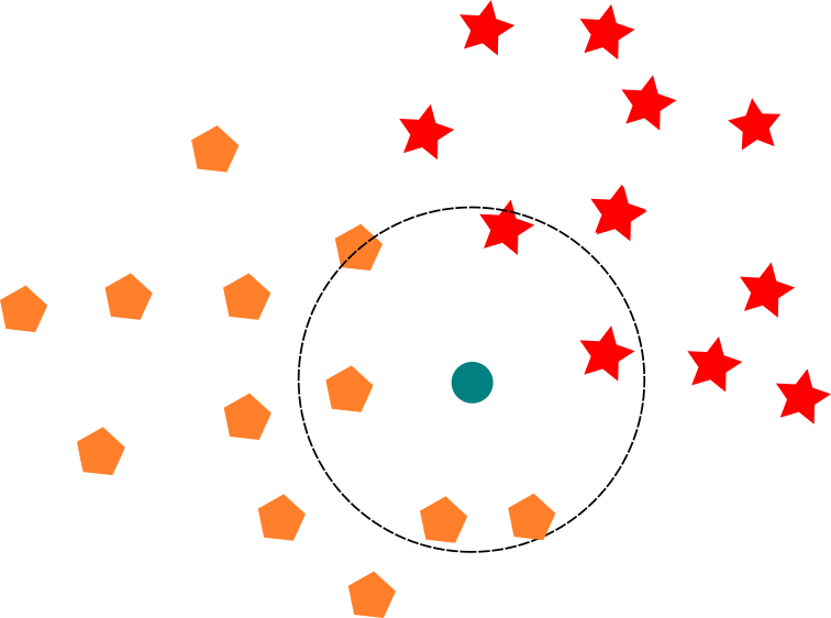
As old saying goes, you are who you surround yourself with. This idea even has mathematical interpretation. In N-dimensional space, points that are closer to each other are more similar, then ones that stand apart. This is the assumption that KNN algorithm makes. It tries to find K nearest known points or samples, also called “neighbors”, to some unknown sample. Majority class of neighbors defines class of the unknown sample.

Nearest neighbors defines class of unknown sample

To came from this idea to implementation, we need to define how to find closest points.

Closest Points

We need to somehow measure distance between samples in order to find closest (hence similar) neighbors. Turned out there are quite a few metrics we can use:

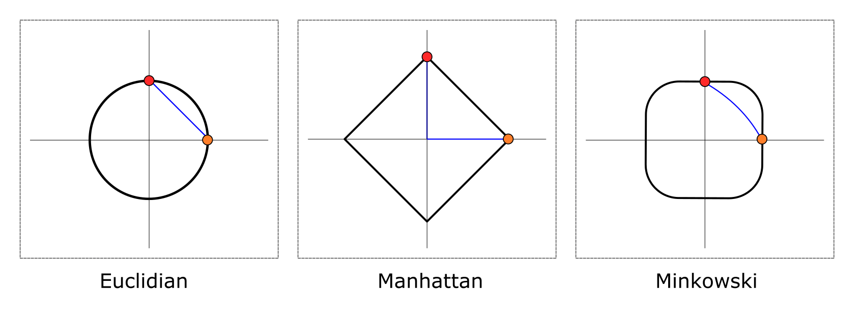
Euclidean Distance - straight-line distance between two points
Manhattan (City Block) Distance - distance between two points traversed along one axis at the time at right angle
Minkowski Distance - Generalization of Euclidean and Manhattan distances
scikit-learn supports other metrics as well

Different distance metrics and their boundaries

Distance metrics and their boundaries in 2D

Euclidean and Manhattan distances are two the most popular distance metrics:

D(x, y)_{euclidean} = \sqrt{\sum_{i=1}^n (x_i-y_i)^2}

D(x, y)_{manhattan} = \sum_{i=1}^n |x_i-y_i|

where $x=(x_1, x_2, ..., x_n)$ and $y=(y_1, y_2, ..., y_n)$ are two points in the N-dimensional space.

Minkowski distance incorporates both Euclidean (when p is 2) and Manhattan (when p is 1) distances and gives additional degree of flexibility via p param:

D(x, y)_{minkowski} = \left(\sum_{i=1}^n (|x_i-y_i|)^p\right)^\frac{1}{p}

These distance metrics are intuitive and fast to compute.

However, all features or dimensions are treated the same way. This may be an issue if features have values in different scales. For example,

customer age value is normally between 18 and 100
annual income values lies between 20,000 and 200,000 (and sometimes goes far beyond)

When calculating distance metrics, this leads to a situation when major part of similarity actually comes from large scale-value features (like annual income). As a result, the rest of the features will be almost neglected and won’t be really taken into account during similarity checking.

Standardization

Ignoring small-scale features in the similarity checking is rarely a desired effect. We would like rather to avoid it to get real neighbors of our sample.

We can try to rescale all features to the same range (0-1, for example). This will standardize or normalize features and let them have the same influence in the distance calculations.

Z = \frac{x - \overline{x}}{S}

where $x$ is sample feature value, $\overline{x}$ is a feature mean and $S$ is a feature standard deviation.

$Z$ is a standard score (or z-score) of the sample feature value. It’s a dimensionless quantity and it shows how “unusual” or far sample feature value from the feature mean (which is usual or expected value).

Though normalization changes values of features, it doesn’t change feature distribution shape.

Dense Dataset

We assume that similar samples are close in the N-dimensional feature space. Is this always a case?

Turned out that with growing number of dimensions (or features), number of samples should grow exponentially in order to keep the same density of sample points in the space. High-dimensional space contains far more actual space between points than our intuition may suggest.

This may lead to a situation when distance to neighbors across all feature axis are just slightly bigger than average distance between points. In sparse high-dimensional feature space we are loosing our notion of nearest points.

This is the reason why ratio of features to samples is important for KNN algorithm.

Neighborhood Size

Effectiveness of applying KNN depends greatly on choosing appropriate size of neighborhood a.k.a K hyperparam. In turn this choice is determined by dataset. It’s usual to see K in range from 1 to 20 (5 is default size in scikit-learn).

Smaller value of K adds more sensitivity and variance. For noisy datasets this means that given a slightly adjusted dataset we may get a different neighbors.

Increasing K hyperparam adds more bias to KNN results and smoother decision boundaries. If K param value is too big, KNN will loose its ability to find local structures in the dataset.

In general, neighborhood size is subject of hyperparam tuning. Final decision should be validated on separated validation dataset.

Applications

You may find KNN-based classificators and regressors which is a trivial application of KNN idea. Let’s review a few less obvious applications where KNN shines even better.

Feature Engineering

KNN is able to identify local structures in the dataset. This information is useful clue itself and local structure labels may be used in classification/regression pipeline as an additional feature.

Neighbors in Embeddings

KNN algorithm becomes useful when you have embeddings - samples projected into lower dimensional latent space. In embedding space distance means similarity and KNN can suggest similar items. This is especially useful for recommendation systems. In that case, nearest neighbor search can be optimized further by leveraging locality-sensitive hashing, for instance.

Anomaly Detection

Distances to K nearest neighbors can be viewed as an estimation of local density. If distance is relatively large, this implies that density is low and sample is likely to be an outlier.

Summary

I hope we shed a bit of light on theoretical aspects of K-Nearest Neighbor algorithm and proved that this pure idea is still useful after decades of being formulated.

Blog